GDP components over time and among countries

The main components of gross domestic product, GDP are personal consumption (C), business investment (I), government spending (G) and net exports (exports - imports).

The GDP data we will look at is from the United Nations’ National Accounts Main Aggregates Database, which contains estimates of total GDP and its components for all countries from 1970 to today.

We will look at how GDP and its components have changed over time, and compare different countries and how much each component contributes to that country’s GDP.

UN_GDP_data  <-  read_excel(here::here("data", "Download-GDPconstant-USD-countries.xls"), # Excel filename
                sheet="Download-GDPconstant-USD-countr", # Sheet name
                skip=2) # Number of rows to skip

Tidy data in long format, and express express all figures in billions

# Contentrate the year columns
tidy_GDP_data  <-  UN_GDP_data %>% 
  pivot_longer(cols = 4:51,
               names_to = "year") %>% 
  mutate(value=value/1e9) 

glimpse(tidy_GDP_data)

## Rows: 176,880
## Columns: 5
## $ CountryID     <dbl> 4, 4, 4, 4, 4, 4, 4, 4, 4, 4, 4, 4, 4, 4, 4, 4, 4, 4, 4,~
## $ Country       <chr> "Afghanistan", "Afghanistan", "Afghanistan", "Afghanista~
## $ IndicatorName <chr> "Final consumption expenditure", "Final consumption expe~
## $ year          <chr> "1970", "1971", "1972", "1973", "1974", "1975", "1976", ~
## $ value         <dbl> 5.559069, 5.332823, 5.197066, 5.746510, 6.147288, 6.3217~

# Let us compare GDP components for these 3 countries
country_list <- c("United States","India", "Germany")

To graph GDP components over time, we take a look at the data and look at out GDP component names (see indicator list).

# Skim the data
skimr::skim(tidy_GDP_data)

Table 1: Data summary

Name	tidy_GDP_data
Number of rows	176880
Number of columns	5
_______________________
Column type frequency:
character	3
numeric	2
________________________
Group variables	None

Variable type: character

skim_variable	n_missing	complete_rate	min	max	empty	n_unique	whitespace
Country	0	1	4	34	0	220	0
IndicatorName	0	1	17	88	0	17	0
year	0	1	4	4	0	48	0

Variable type: numeric

skim_variable	n_missing	complete_rate	mean	sd	p0	p25	p50	p75	p100	hist
CountryID	0	1.00	439.17	254.06	4.00	214.00	440.0	660.0	894.00	▇▇▇▇▆
value	15421	0.91	72.19	447.45	-567.67	0.36	2.5	17.9	17348.63	▇▁▁▁▁

# Get GDP component names by gettting unique values 
unique(tidy_GDP_data$IndicatorName)

##  [1] "Final consumption expenditure"                                                           
##  [2] "Household consumption expenditure (including Non-profit institutions serving households)"
##  [3] "General government final consumption expenditure"                                        
##  [4] "Gross capital formation"                                                                 
##  [5] "Gross fixed capital formation (including Acquisitions less disposals of valuables)"      
##  [6] "Exports of goods and services"                                                           
##  [7] "Imports of goods and services"                                                           
##  [8] "Gross Domestic Product (GDP)"                                                            
##  [9] "Agriculture, hunting, forestry, fishing (ISIC A-B)"                                      
## [10] "Mining, Manufacturing, Utilities (ISIC C-E)"                                             
## [11] "Manufacturing (ISIC D)"                                                                  
## [12] "Construction (ISIC F)"                                                                   
## [13] "Wholesale, retail trade, restaurants and hotels (ISIC G-H)"                              
## [14] "Transport, storage and communication (ISIC I)"                                           
## [15] "Other Activities (ISIC J-P)"                                                             
## [16] "Total Value Added"                                                                       
## [17] "Changes in inventories"

# Create indicator list to list out target GDP components
indicator_list <- c("Gross capital formation",
                    "Exports of goods and services",
                    "Imports of goods and services",
                    "Household consumption expenditure (including Non-profit institutions serving households)",
                    "General government final consumption expenditure")

library(scales)

## Warning: package 'scales' was built under R version 4.1.1

## 
## Attaching package: 'scales'

## The following object is masked from 'package:mosaic':
## 
##     rescale

## The following object is masked from 'package:purrr':
## 
##     discard

## The following object is masked from 'package:readr':
## 
##     col_factor

# Filter target countries and gdp component
country_list_gdp <- tidy_GDP_data%>%
  filter(Country %in% country_list,IndicatorName %in% indicator_list )

# Plot the line graph, grouped by GDP indicator, faceted by country
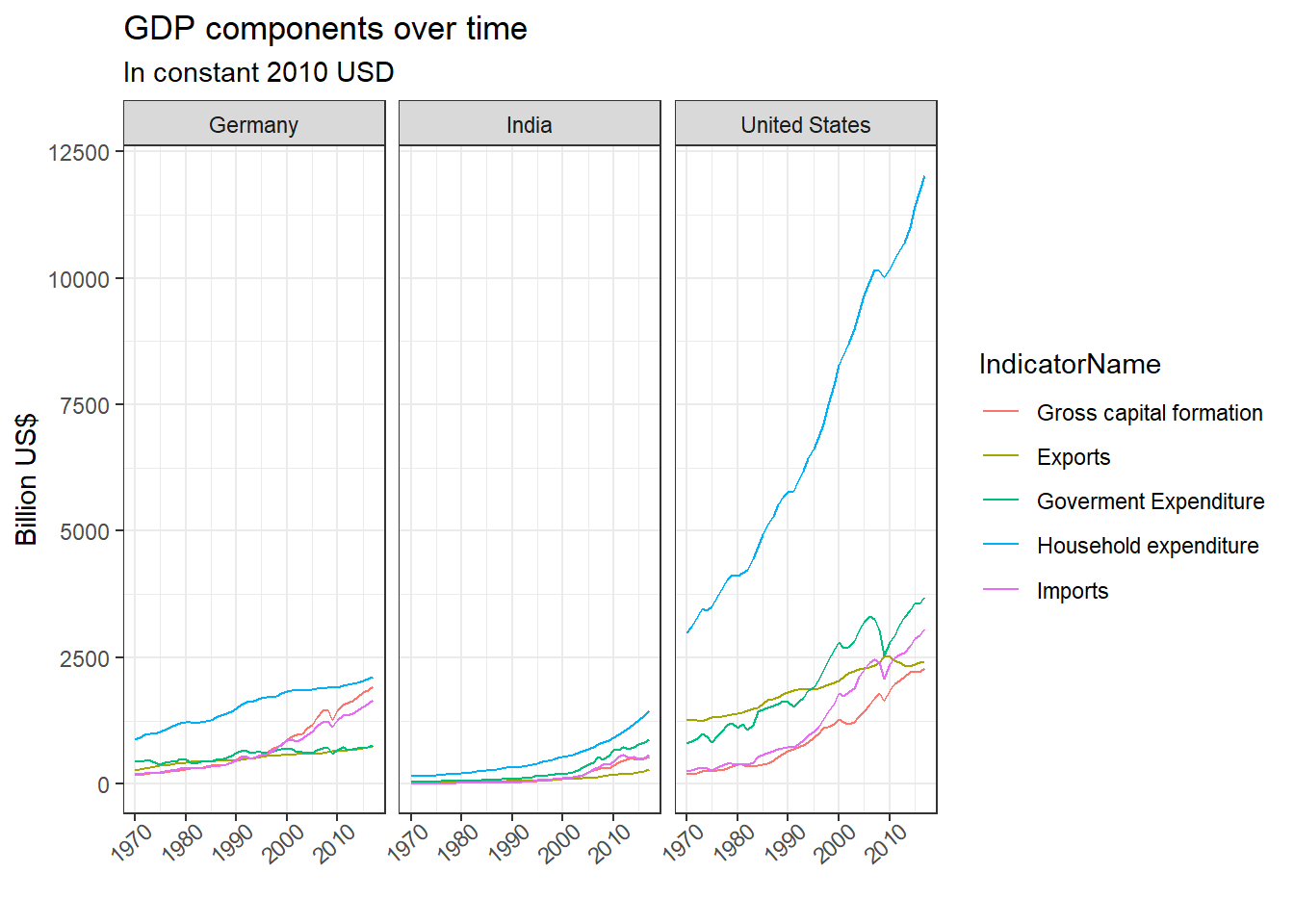
ggplot(country_list_gdp,aes(x = as.numeric(year), group = IndicatorName))+
  geom_line(aes(y = value, color = IndicatorName))+
  facet_wrap(~Country)+
  theme_bw()+
  # Adjust legend position to the right
  theme(legend.position = "right",
        # Adjust x axis by turing 40 degrees to avoid overlapping
        axis.text.x = element_text(angle = 40, hjust = 0.8))+
  # Break the x axis to intervals of 5
  scale_x_continuous(breaks = scales::pretty_breaks(n=5),)+
  # Label title and axis
  labs(title="GDP components over time",
       subtitle="In constant 2010 USD",
       x="",
       y="Billion US$")+
  # Order the labels for gdp component
  scale_color_discrete(labels = c("Gross capital formation",
                                "Exports",
                                "Goverment Expenditure",
                                "Household expenditure",
                                "Imports")
      )

GDP is the sum of Household Expenditure (Consumption C), Gross Capital Formation (business investment I), Government Expenditure (G) and Net Exports (exports - imports). Below calculate GDP with the sum of the GDP components, and compare with the GDP provided in the indicator Gross Domestic Product (GDP) in the dataframe. WE will be plotting GDP and its own breakdown at constant 2010 prices in US Dollars.

# Expand the columns by GDP component names
tidy_gdp_wider <- tidy_GDP_data%>%
  pivot_wider(names_from = IndicatorName, values_from = value)

# Calulate net export by export minus import  
tidy_gdp_wider <- tidy_gdp_wider%>%
  mutate(net_export = tidy_gdp_wider[[indicator_list[2]]] - tidy_gdp_wider[[indicator_list[3]]])

# Calculate GDP with C + I + G + net export
tidy_gdp_wider <- tidy_gdp_wider%>%
  mutate(calc_gdp = tidy_gdp_wider[[indicator_list[1]]]+ 
                        tidy_gdp_wider[[indicator_list[4]]]+
                        tidy_gdp_wider[[indicator_list[5]]]+
                        tidy_gdp_wider[["net_export"]],
         # Calculate the percentage of GDP components to calculated GDP
         prc_of_gdp_gross_capital = tidy_gdp_wider[[indicator_list[1]]]/calc_gdp * 100,
         prc_of_gdp_house = tidy_gdp_wider[[indicator_list[4]]]/calc_gdp * 100,
         prc_of_gdp_gov = tidy_gdp_wider[[indicator_list[5]]]/calc_gdp * 100,
         prc_of_gdp_net_exp = tidy_gdp_wider[["net_export"]]/calc_gdp * 100)


# GDP component list with net export
indicator_list_2 <- c("Gross capital formation",
                      "Household consumption expenditure (including Non-profit institutions serving households)",
                      "General government final consumption expenditure",
                      "net_export")

# Contract the columns by GDP component names
calc_gdp_longer <- tidy_gdp_wider%>%
  pivot_longer(cols = 22:26 , names_to = "IndicatorName")

# Filter target countries and perentage GDP components
calc_gdp_longer%>%
  filter(Country %in% country_list)%>%
  filter(IndicatorName %in% c("prc_of_gdp_gross_capital","prc_of_gdp_house","prc_of_gdp_gov","prc_of_gdp_net_exp"))%>%
  # Plot line graph by indicator names facted by country
ggplot(aes(x = as.numeric(year), group = IndicatorName))+
  geom_line(aes(y = value, color = IndicatorName))+
  facet_wrap(~Country)+
  theme_bw()+
  # Adjust legend position
  theme(legend.position = "right",
        # Adjust x axis by turing 40 degrees to avoid overlapping
        axis.text.x = element_text(angle = 40, hjust = 0.8))+
  # Order the labels for gdp component
  scale_color_discrete(labels = c("Goverment Expenditure",
                                "Gross Capital Formation",
                                "Gross Household Expenditure",
                                "Net Export")
      )+
  # Break the x axis to intervals of 5
  scale_x_continuous(breaks = scales::pretty_breaks(n=5))+
  # Label title and axis
  labs(title="GDP and its breakdown at constant 2010 prices in US Dollars",
       x="",
       y="Billion US$")+
  # Format y axis in percentages
  scale_y_continuous(labels = function(y) sprintf("%.1f %%",y))

# Percentage difference between caluclated GDP and actual GDP
tidy_gdp_wider<- tidy_gdp_wider%>%
  mutate(calc_vs_real_gdp = calc_gdp / tidy_gdp_wider[["Gross Domestic Product (GDP)"]]-1 )

The percentage difference changes from year to year depending on how much the factors within the table that we did not use in our calculation contributed to the total GDP.

All three countries have highest proportion of GDP in Household Expenditure and lowest proportion of GDP in Net Exports. India has the highest household consumption proportion compared to Germany and the United States, yet it is decreasing over the years. In contrast, gross capital formation proportion increased significantly over the years. This might be due to India being a developing country where incomes flows towards investment capital consumption from household consumption capital. Germany and the United states showcase similar pattern of all proportion being relatively stable over the years. Both countries are developed countries with stable development, which explains the relatively less volatile proportion changes.